Visual diagnostics for multiply imputed values
Yongshi Deng
2024-01-08
Source:vignettes/web/Visual-diagnostics.Rmd
Visual-diagnostics.Rmd1. Introduction
It is crucial to assess the plausibility of imputations before doing
an analysis. The mixgb package provides several visual
diagnostic functions using ggplot2 to compare multiply
imputed values versus observed data.
1.1 Inspecting imputed values
We will demonstrate these functions using the
nhanes3_newborn dataset. In the original data, almost all
missing values occurred in numeric variables. Only seven observations
are missing in the binary factor variable HFF1.
library(mixgb)
colSums(is.na(nhanes3_newborn))
#> HSHSIZER  HSAGEIR    HSSEX DMARACER DMAETHNR DMARETHN  BMPHEAD BMPRECUM
#>        0        0        0        0        0        0      124      114
#>   BMPSB1   BMPSB2   BMPTR1   BMPTR2    BMPWT   DMPPIR     HFF1     HYD1
#>      161      169      124      167      117      192        7        0
In order to visualize some imputed values for other types of
variables, we create some extra missing values in HSHSIZER
(integer), HSAGEIR (integer), HSSEX (binary
factor), DMARETHN (multiclass factor) and HYD1
(Ordinal factor) under the missing completely at random (MCAR)
mechanism.
withNA.df <- createNA(data = nhanes3_newborn, var.names = c("HSHSIZER", "HSAGEIR", "HSSEX", "DMARETHN", "HYD1"), p = 0.1)
colSums(is.na(withNA.df))
#> HSHSIZER  HSAGEIR    HSSEX DMARACER DMAETHNR DMARETHN  BMPHEAD BMPRECUM
#>      211      211      211        0        0      211      124      114
#>   BMPSB1   BMPSB2   BMPTR1   BMPTR2    BMPWT   DMPPIR     HFF1     HYD1
#>      161      169      124      167      117      192        7      211
We then impute this dataset using mixgb() with default
settings. After completion, a list of five imputed datasets is assigned
to imputed.data. Each imputed dataset will have the same
dimension as the original data.
imputed.data <- mixgb(data = withNA.df, m = 5)By using the function show_var(), we can see the
multiply imputed values of the missing data for a given variable. The
function returns a data.table of m columns, each of which
represents a set of imputed values for the variable of interest. Note
that the output of this function only includes the imputed values of
missing entries in the specified variable.
show_var(imputation.list = imputed.data, var.name = "BMPHEAD", original.data = withNA.df)
#>            m1       m2       m3       m4       m5
#>   1: 43.69530 43.06142 43.46896 43.18378 43.72390
#>   2: 43.54941 44.44894 43.88666 44.52724 44.17919
#>   3: 42.96304 43.42857 44.05237 43.16604 42.83355
#>   4: 45.85104 47.08269 46.15845 46.21148 45.83071
#>   5: 45.27668 45.37537 44.76131 45.77869 45.60131
#>  ---
#> 120: 44.97638 45.05478 45.71369 45.38212 45.09203
#> 121: 44.50610 44.79557 44.61496 44.91100 45.13340
#> 122: 41.64592 41.01516 41.44185 41.04568 42.05811
#> 123: 45.13840 45.38054 44.97987 43.91048 44.64847
#> 124: 47.62844 45.49401 46.78232 46.15891 45.61115
show_var(imputation.list = imputed.data, var.name = "HFF1", original.data = withNA.df)
#>    m1 m2 m3 m4 m5
#> 1:  2  2  2  2  2
#> 2:  2  2  2  2  2
#> 3:  2  2  2  2  2
#> 4:  2  2  2  2  2
#> 5:  1  1  1  1  1
#> 6:  2  2  2  2  1
#> 7:  2  2  2  2  1
2 Visual diagnostics plots
The mixgb package provides the following visual
diagnostics functions:
Single variable:
plot_hist(),plot_box(),plot_bar();Two variables:
plot_2num(),plot_2fac(),plot_1num1fac();Three variables:
plot_2num1fac(),plot_1num2fac().
Each function returns m+1 panels that enable a
comparison between the observed data and m sets of imputed
values for the missing data.
2.1 Single variable
Only imputed values of missing entries in the specified variable will
be plotted in panels m1 to m5. An error
message will be displayed if the variable is fully observed and there
are no missing entries to impute.
2.1.1 Numeric
We can plot an imputed numeric variable by histogram or boxplot.
-
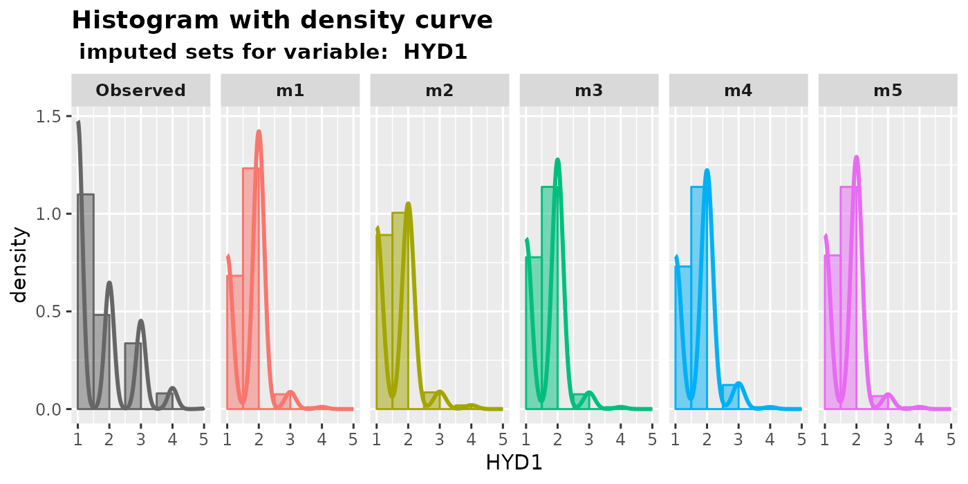
plot_hist(): plot histograms with density curves.Histograms are a useful tool for displaying the distribution of numeric data. Users can examine the shapes of the histograms to identify any unusual patterns in the imputed values. If the data is missing completely at random (MCAR), we would expect the distribution of imputed values to be the same as that of the observed values. However, if the data is missing at random (MAR), the distributions of observed and imputed values can be quite different. Nevertheless, it is still worth plotting the imputed data, as any unusual values may indicate that the imputation procedure is unsatisfactory.
plot_hist(
  imputation.list = imputed.data, var.name = "BMPHEAD",
  original.data = withNA.df
)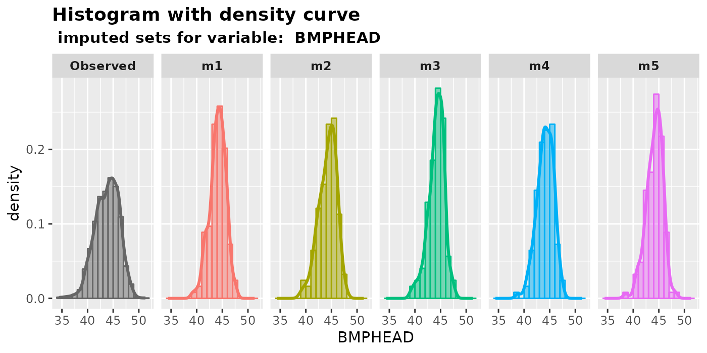
-
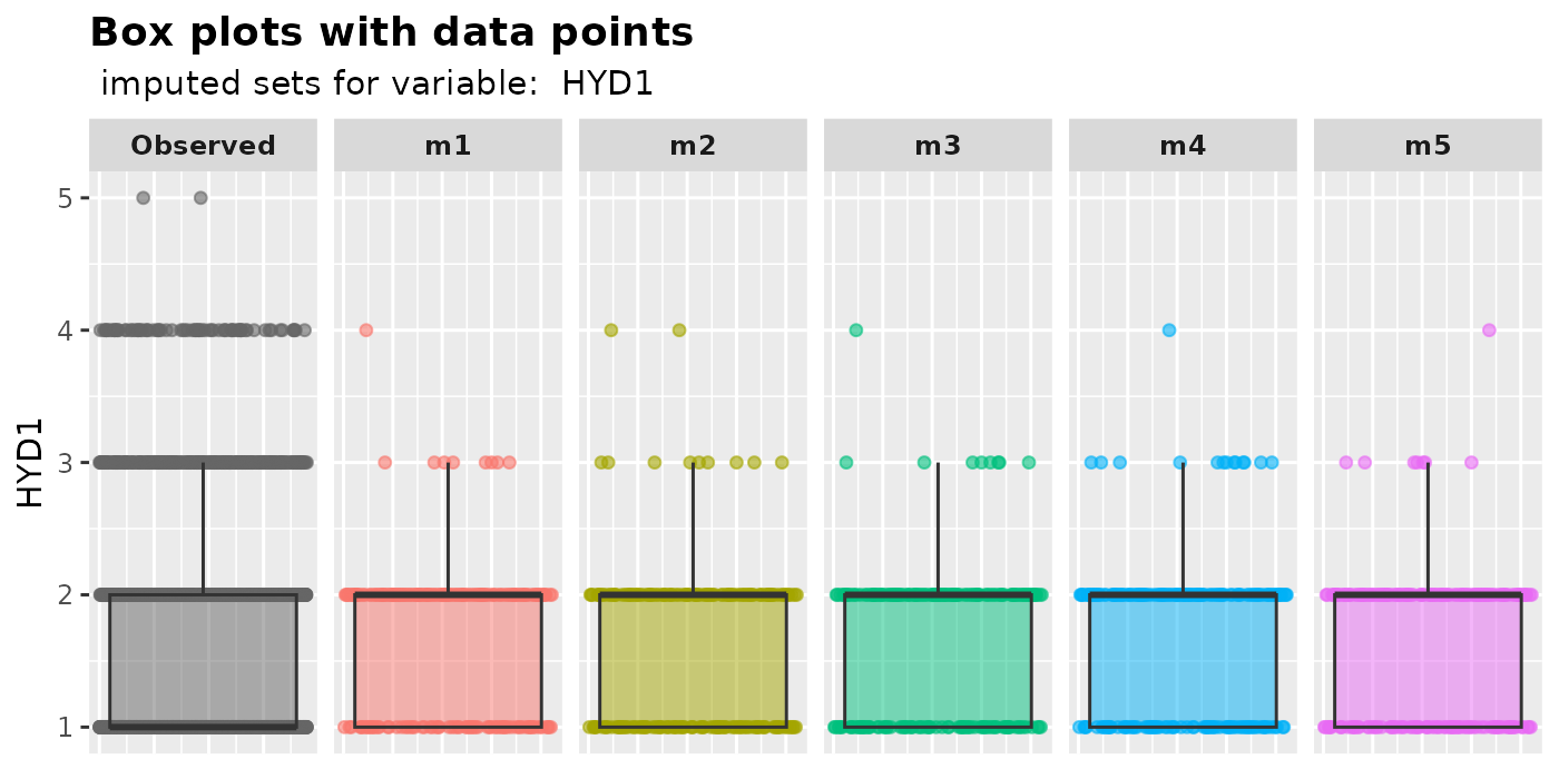
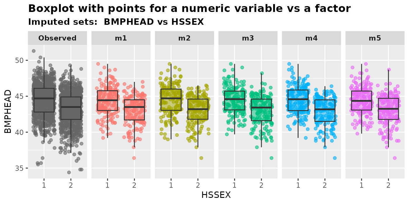
plot_box(): plot box plots with overlaying data points.Users can use
plot_box()to compare the median, lower and upper quantiles of imputed values with those of the observed values. The plot also visually displays the disparity in counts between observed and missing values in the variable of interest.plot_box( imputation.list = imputed.data, var.name = "BMPHEAD", original.data = withNA.df )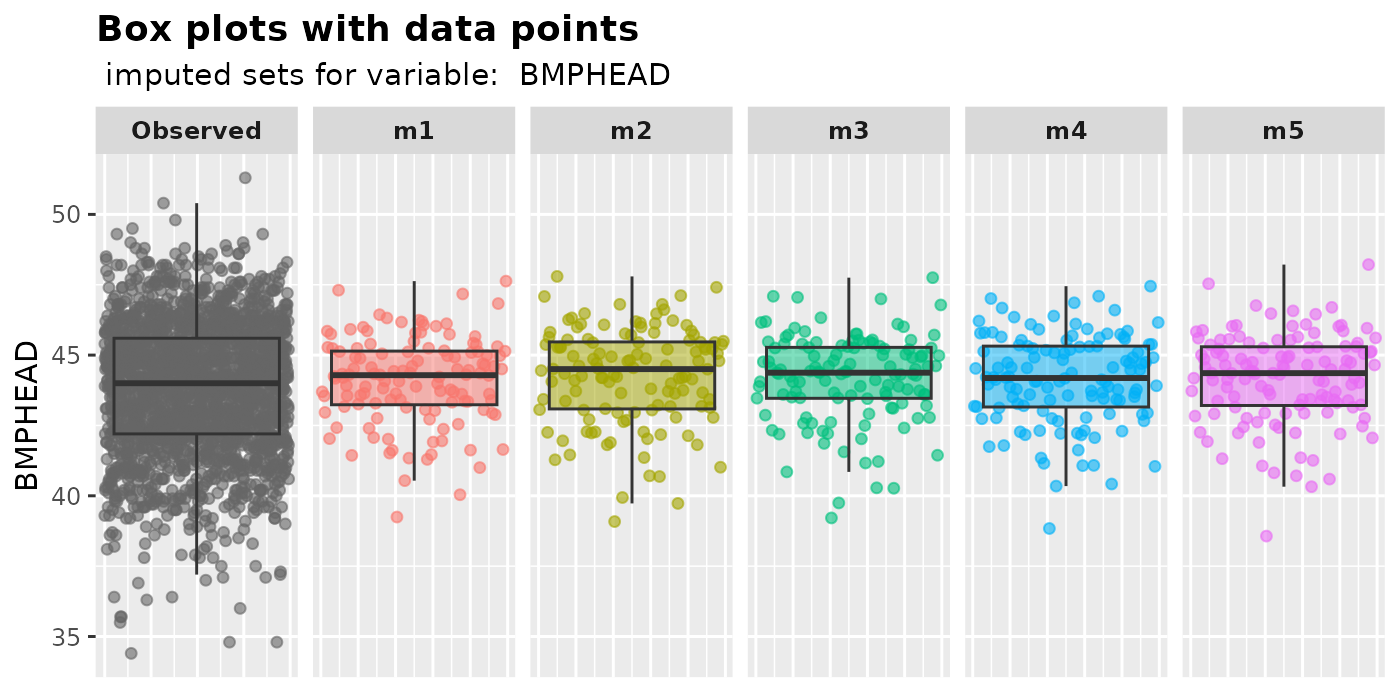
2.1.2 Factor
-
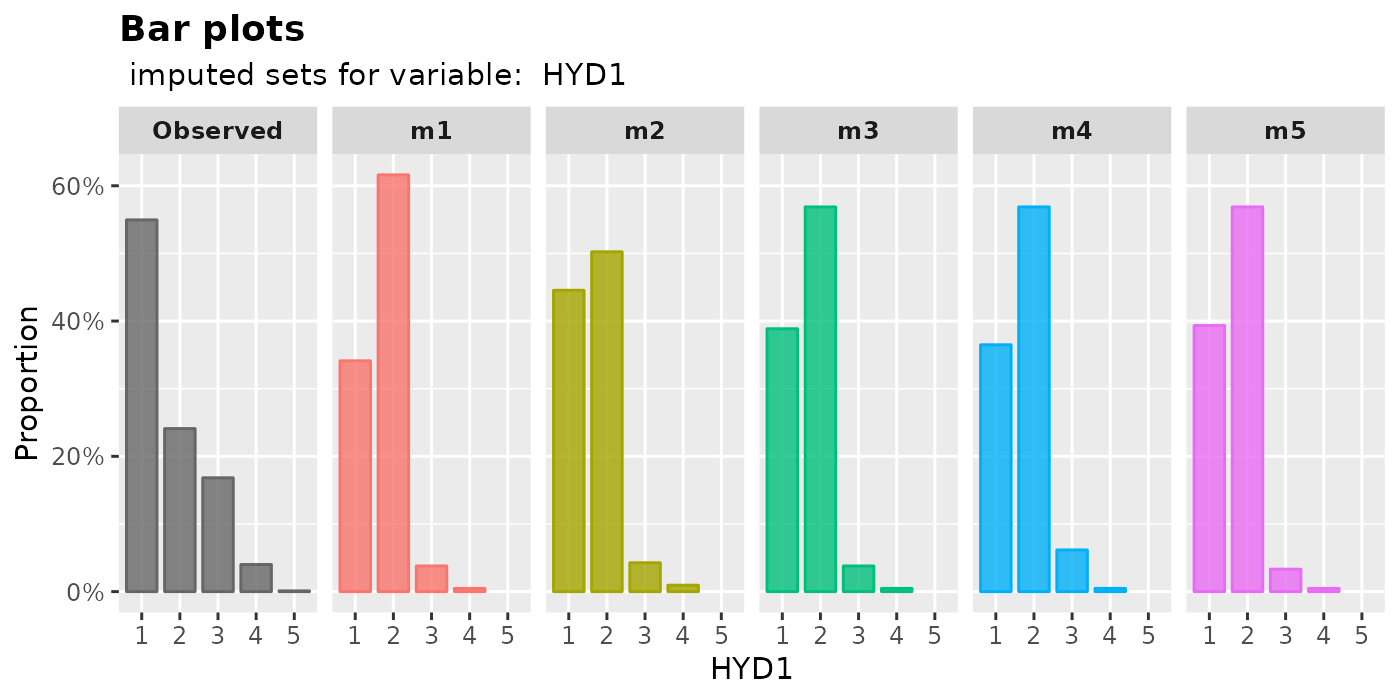
plot_bar(): plot bar plotsThe proportion of each level in a factor will be shown by
plot_bar().plot_bar( imputation.list = imputed.data, var.name = "HSSEX", original.data = withNA.df )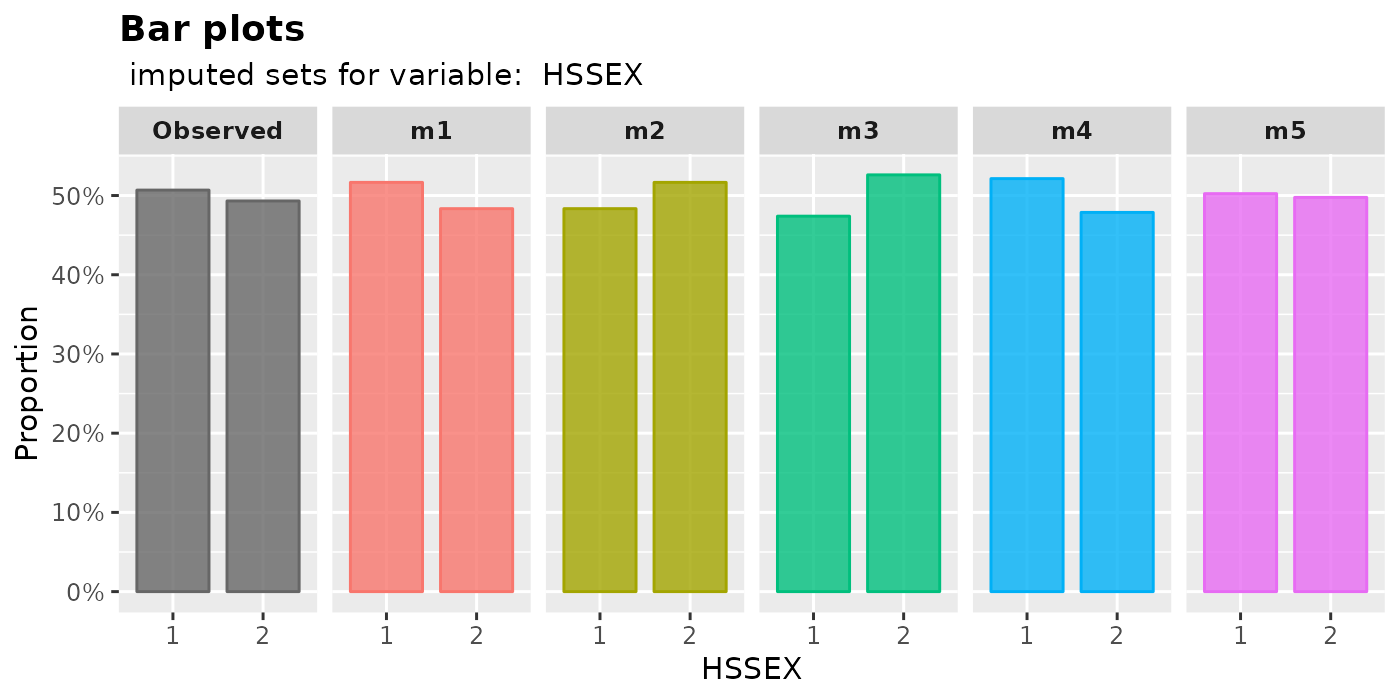
plot_bar(
  imputation.list = imputed.data, var.name = "DMARETHN",
  original.data = withNA.df
)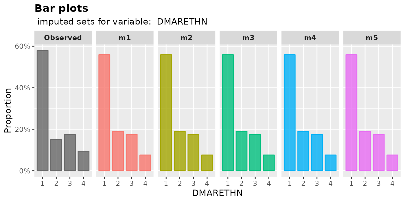
2.1.3 Integer
Users have the flexibility to choose how to treat integer variables when generating a plot, as they can be viewed either as numeric or factor variables. To plot an imputed integer variable, users can use one of the following functions based on their preferred representation:
plot_hist(): plot histograms with density curvesplot_box(): plot box plot with overlaying data points-
plot_bar(): plot bar plot (treat an integer variable as a factor)plot_hist( imputation.list = imputed.data, var.name = "HSHSIZER", original.data = withNA.df )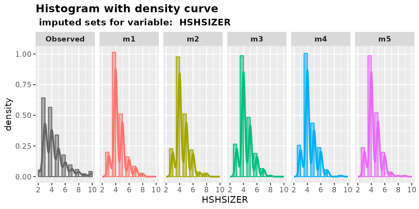
plot_box(
  imputation.list = imputed.data, var.name = "HSHSIZER",
  original.data = withNA.df
)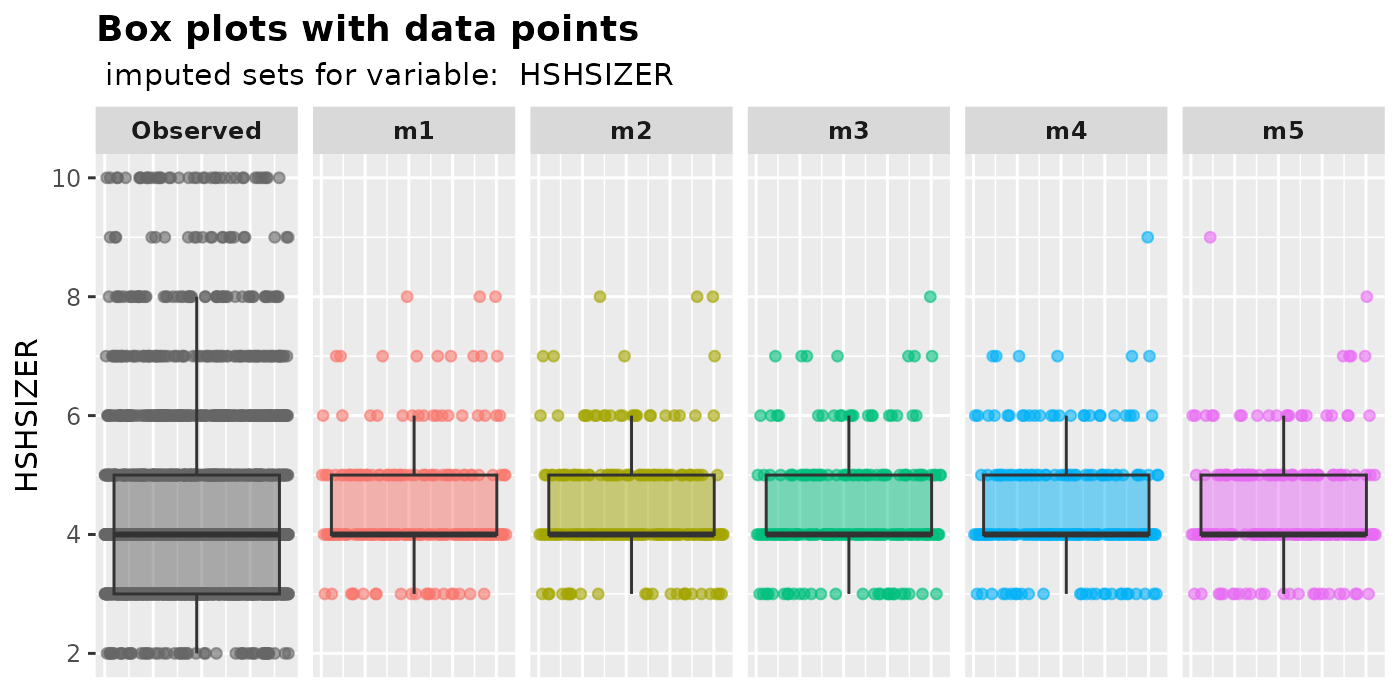
plot_bar(
  imputation.list = imputed.data, var.name = "HSHSIZER",
  original.data = withNA.df
)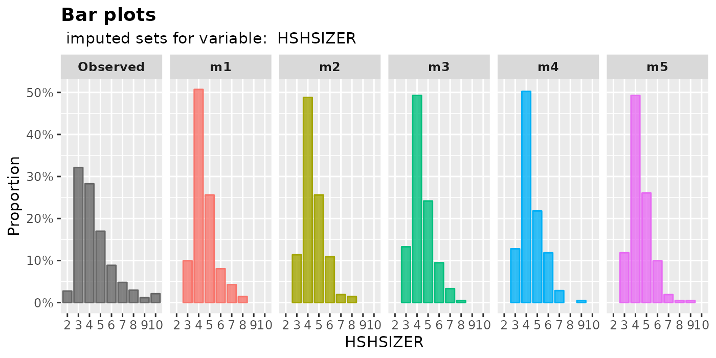
2.1.4 Ordinal factor
By default, the function mixgb() does not convert
ordinal factors to integers. Therefore, we may simply plot ordinal
factors as factors (see Section 2.1.2).
However, setting ordinalAsInteger = TRUE in
mixgb() may speed up the imputation process, but users must
decide whether to transform them back. If we choose to convert ordinal
factors to integers prior to imputation, the imputed values must be
plotted as if they were integers (see Section 2.1.3).
imputed.data2 <- mixgb(data = withNA.df, m = 5, ordinalAsInteger = TRUE)

plot_bar(
  imputation.list = imputed.data2, var.name = "HYD1",
  original.data = withNA.df
)
plot_hist(
  imputation.list = imputed.data2, var.name = "HYD1",
  original.data = withNA.df
)
plot_box(
  imputation.list = imputed.data2, var.name = "HYD1",
  original.data = withNA.df
)
2.2 Two variables
All of the functions in this section for visualizing the multiply
imputed values of two variables require at least one of the variables in
the original dataset to be incomplete. The imputed values shown in
panels m1 to m5 are those that were originally
missing in one or both of the variables.
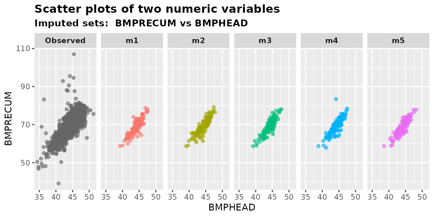
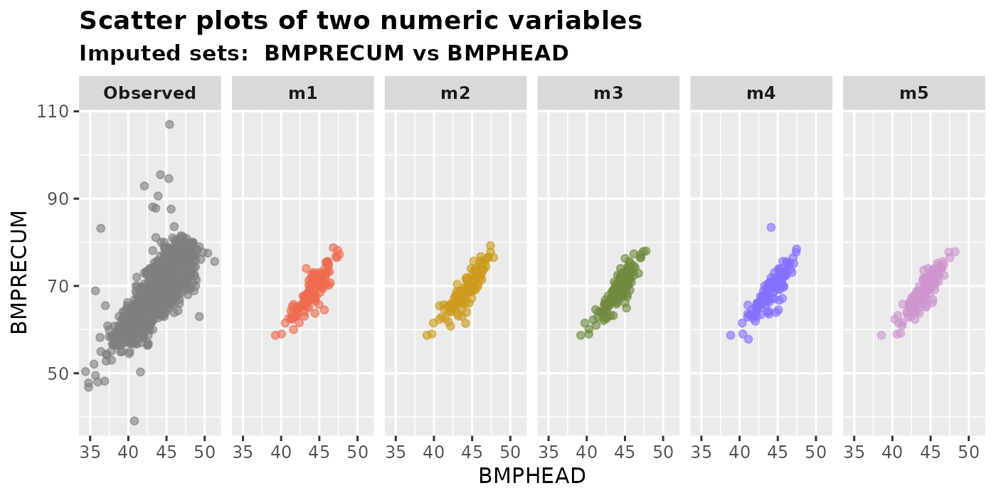
2.2.1 Two numeric variables
We can generate scatter plots of two imputed numeric variables by
using plot_2num(). We can specify the x-axis variable in
var.x and the y-axis variable in var.y.
Users can choose to plot the shapes of different types of missing
values by setting shape = TRUE. We only recommend plotting
the shapes for small datasets. By default, shape = FALSE is
used to expedite the plotting process.
plot_2num(
  imputation.list = imputed.data, var.x = "BMPHEAD", var.y = "BMPRECUM",
  original.data = withNA.df, shape = TRUE
)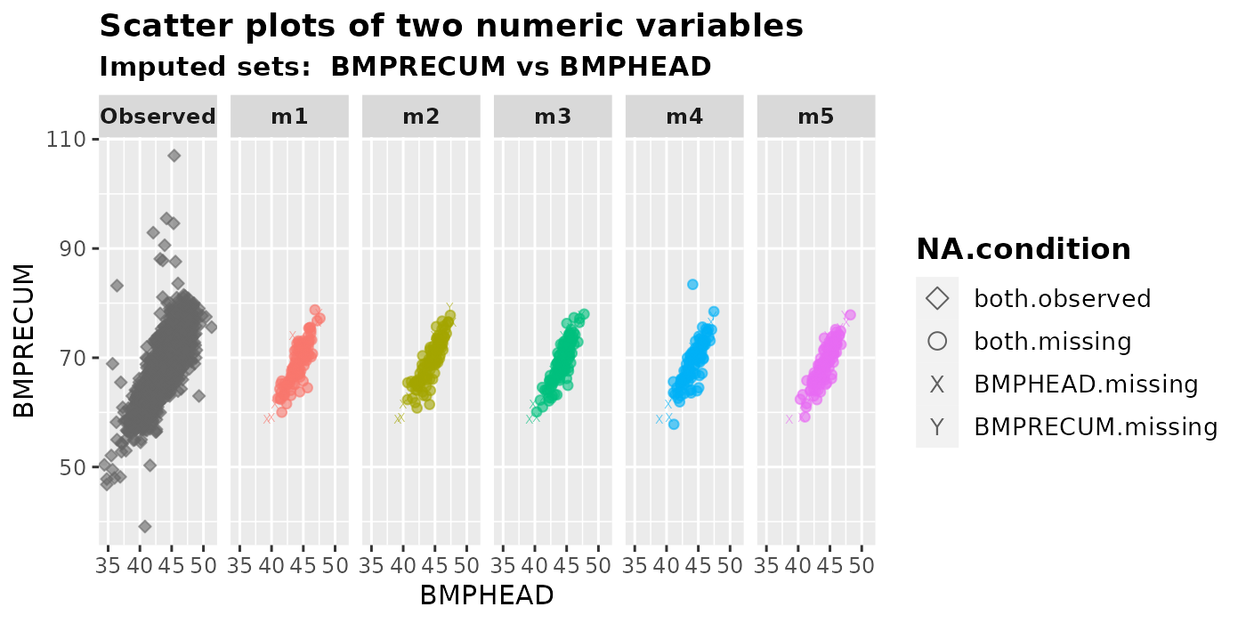
NA.condition represents the following four types of missing values.
both.observed: Bothvar.xandvar.yare observed. This only appears in the first panel -Observed(Shape: diamond).both.missing: Imputed values where bothvar.xandvar.yare originally missing (Shape: circle);var.x.missing: Imputed values wherevar.xis originally missing andvar.yis not (Shape: X);var.y.missing: Imputed values wherevar.yis originally missing andvar.xis not (Shape: Y).
2.2.2 One numeric vs one factor
We can plot a numeric variable versus a factor using
plot_1num1fac(). The output of this function is a box plot
with overlaying points. Users are required to specify a numeric variable
in var.num and a factor in var.fac.
NA.condition is similar to the definition in Section 2.2.1.
plot_1num1fac(
  imputation.list = imputed.data, var.num = "BMPHEAD", var.fac = "HSSEX",
  original.data = withNA.df
)
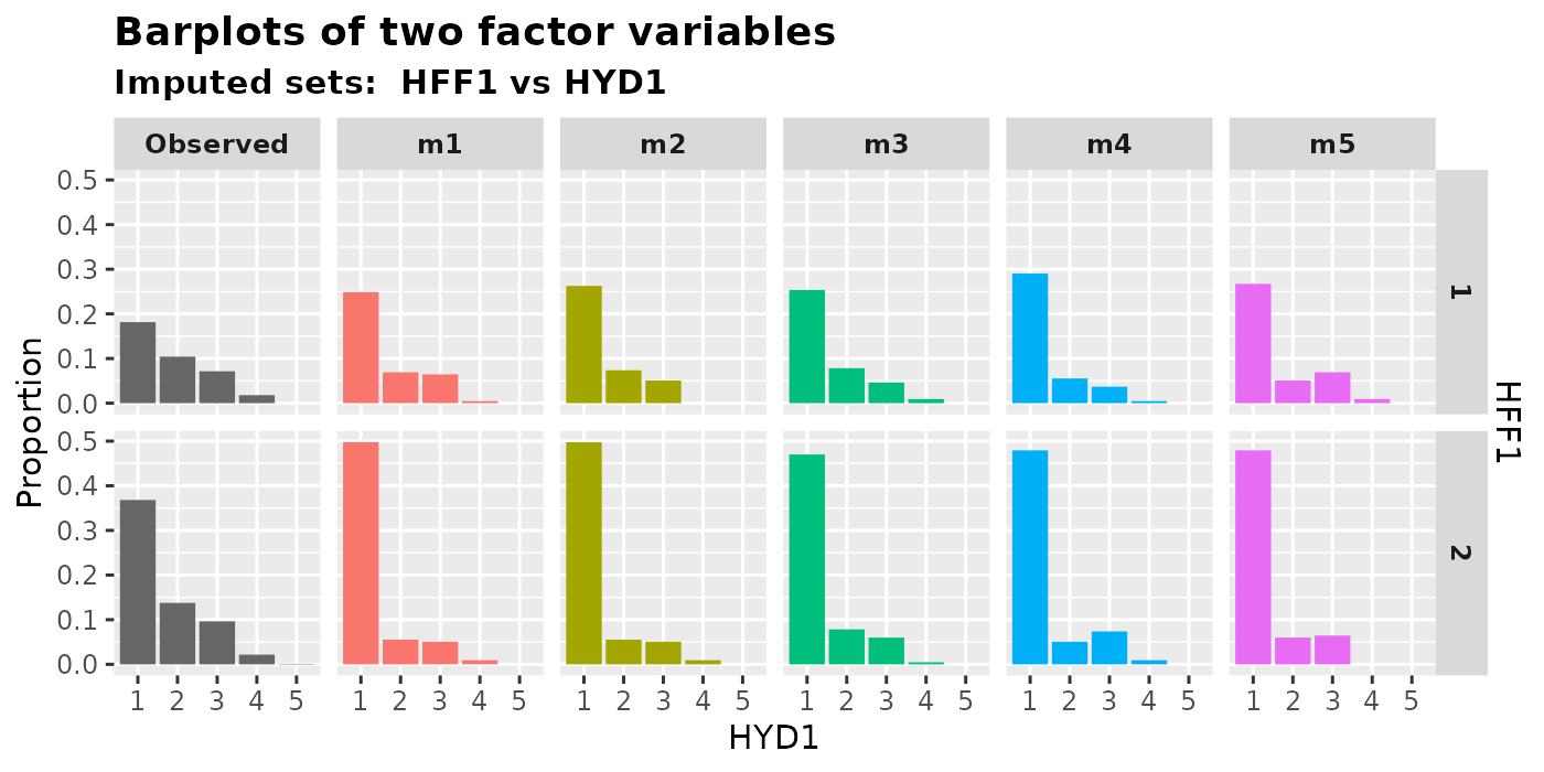
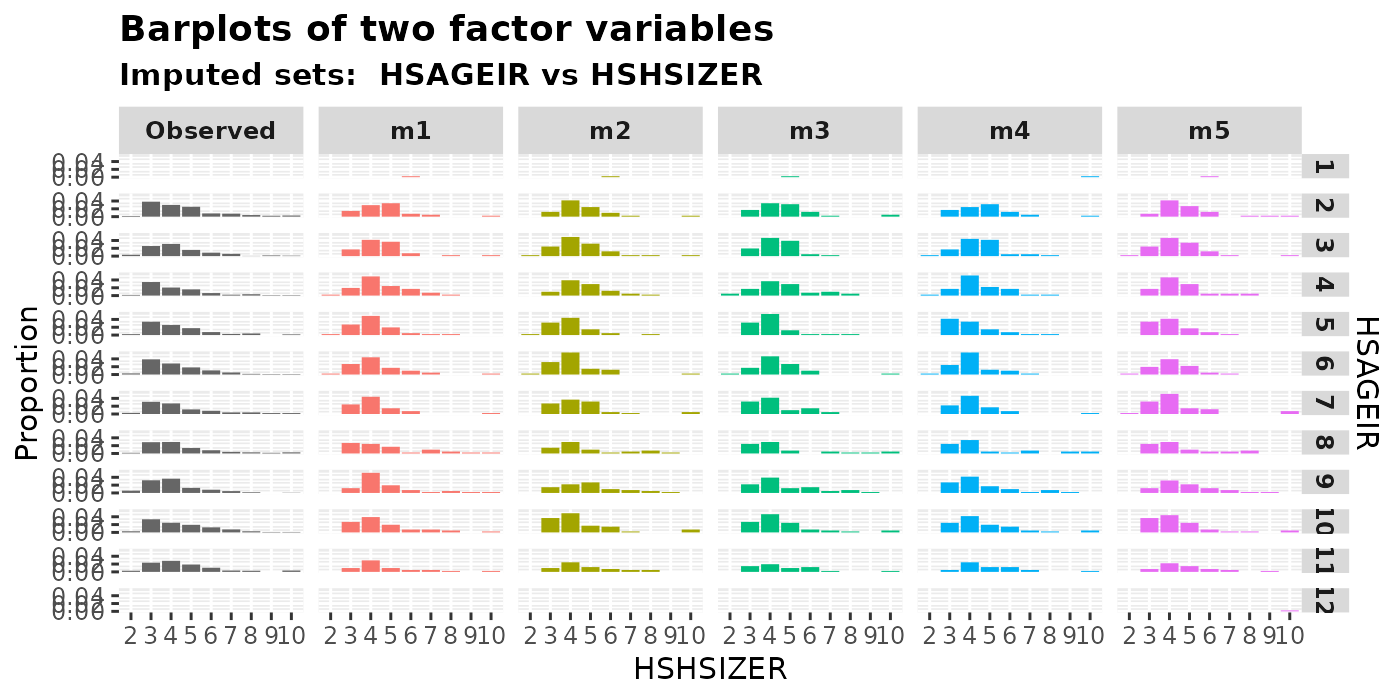
2.2.3 Two factors
We can generate bar plots to show the relationship between two
factors by using plot_2fac().
plot_2fac(
  imputation.list = imputed.data, var.fac1 = "HYD1", var.fac2 = "HFF1",
  original.data = withNA.df
)
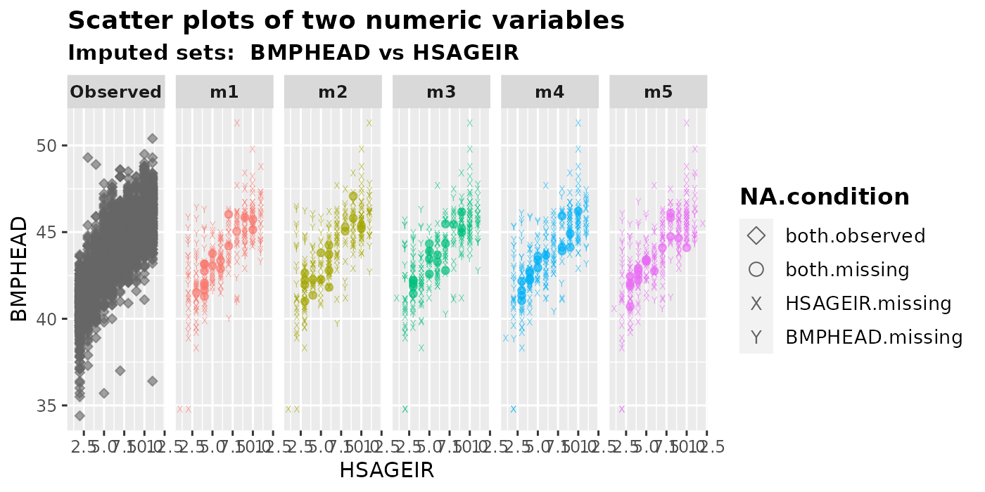
2.2.4 One numeric vs one integer
We can use plot_2num() to visualize the relationship
between a numeric variable and an integer variable. Note that the graphs
would appear differently if the variables var.x and
var.y were swapped.
plot_2num(
  imputation.list = imputed.data, var.x = "BMPHEAD", var.y = "HSAGEIR",
  original.data = withNA.df, shape = TRUE
)
plot_2num(
  imputation.list = imputed.data, var.x = "HSAGEIR", var.y = "BMPHEAD",
  original.data = withNA.df, shape = TRUE
)
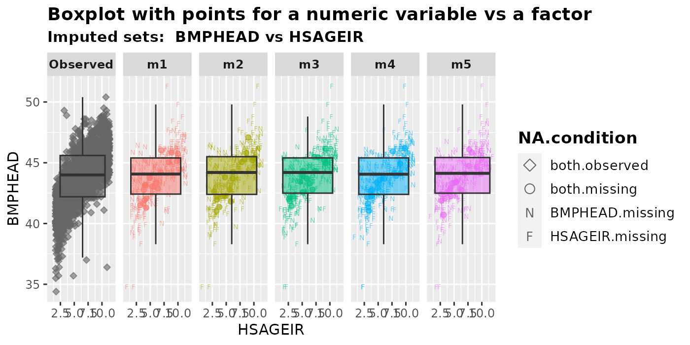
If the integer variable HSAGEIR is to be treated as a
factor rather than a numeric variable, the function
plot 1num1fac() can be used.
plot_1num1fac(
  imputation.list = imputed.data, var.num = "BMPHEAD", var.fac = "HSAGEIR",
  original.data = withNA.df, shape = TRUE
)
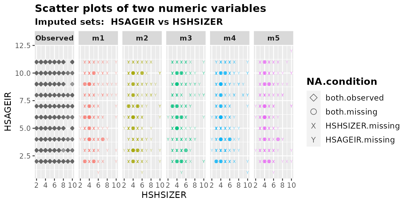
2.2.5 Two integers
We can plot two integer variables using either
plot_2num() ,plot_1num1fac(), or
plot_2fac(). Users should choose the plotting functions
based on the nature of the variable. For example, if an integer variable
age has values between 0 and 110, it may be more convenient
to treat age as numeric rather than a factor. If, on the
other hand, an integer variable has just a few unique values (such as 1,
2, 3), it may be preferable to be plotted as a factor. In this dataset,
there are only two variables of integer type -
HSHSIZER(household size) and HSAGEIR(baby’s
age ranging from 2 to 11 months). Although there is no expected
relationship between these two, we still create a plot for demonstration
purposes.
plot_2num(
  imputation.list = imputed.data, var.x = "HSHSIZER", var.y = "HSAGEIR",
  original.data = withNA.df, shape = TRUE
)
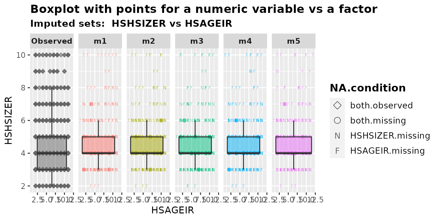
plot_1num1fac(
  imputation.list = imputed.data, var.num = "HSHSIZER", var.fac = "HSAGEIR",
  original.data = withNA.df, shape = TRUE
)
plot_2fac(
  imputation.list = imputed.data, var.fac1 = "HSHSIZER", var.fac2 = "HSAGEIR",
  original.data = withNA.df
)
2.3 Three variables
To plot the multiply imputed values of three variables, at least one of them has to be incomplete in the original dataset.
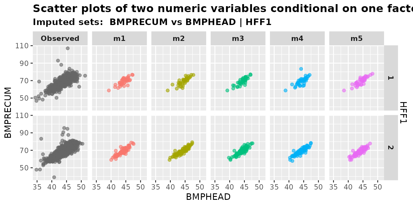
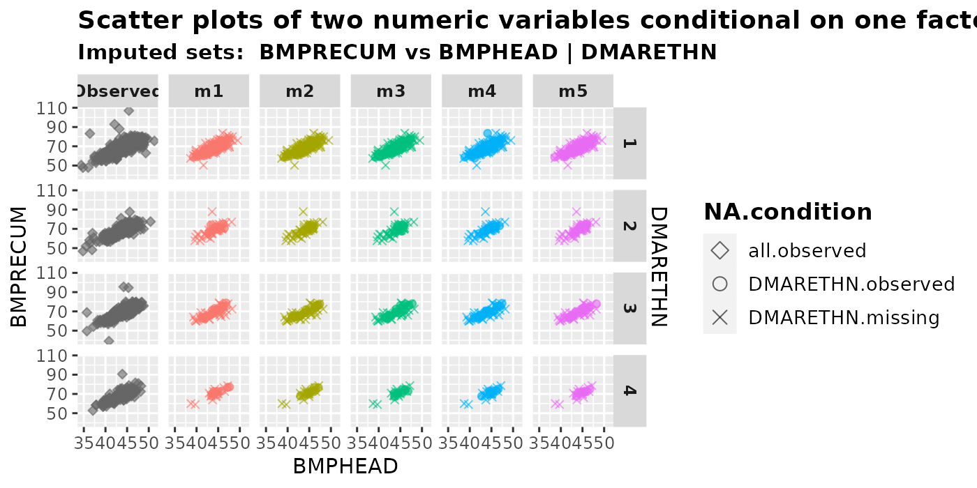
2.3.1 Two numeric variables conditional on one factor
We can generate a scatter plot of two numeric variables when
conditioned on a factor by using plot_2num1fac(). The
variable for the x-axis should be specified in var.x,
whereas the variable for the y-axis should be specified in
var.y. The factor on which we want to condition is
con.fac.
plot_2num1fac(
  imputation.list = imputed.data, var.x = "BMPHEAD", var.y = "BMPRECUM",
  con.fac = "HFF1", original.data = withNA.df
)
When we have three variables, there are \(2^3\) different types of missing patterns.
These patterns consist of all possible combinations of zero to three
variables missing. However, attempting to differentiate all eight types
of missingness in the same plot can be challenging, particularly when
working with large datasets. Therefore, we have decided to display the
following three types of missing patterns
(NA.condition) in the plot when
shape = TRUE.
NA.condition represents the following three types of missing values.
all.observed: Observations where all three variables are observed. This only appears in the first panel -Observed.-
con.fac.observed: Imputed values wherecon.facis originally observed.(These points are originally missing in either
var.xorvar.yor both) con.fac.missing: imputed values wherecon.facis originally missing. (These points can be originally observed, or missing in eithervar.xorvar.yor both)
plot_2num1fac(
  imputation.list = imputed.data, var.x = "BMPHEAD", var.y = "BMPRECUM",
  con.fac = "DMARETHN", original.data = withNA.df, shape = TRUE
)
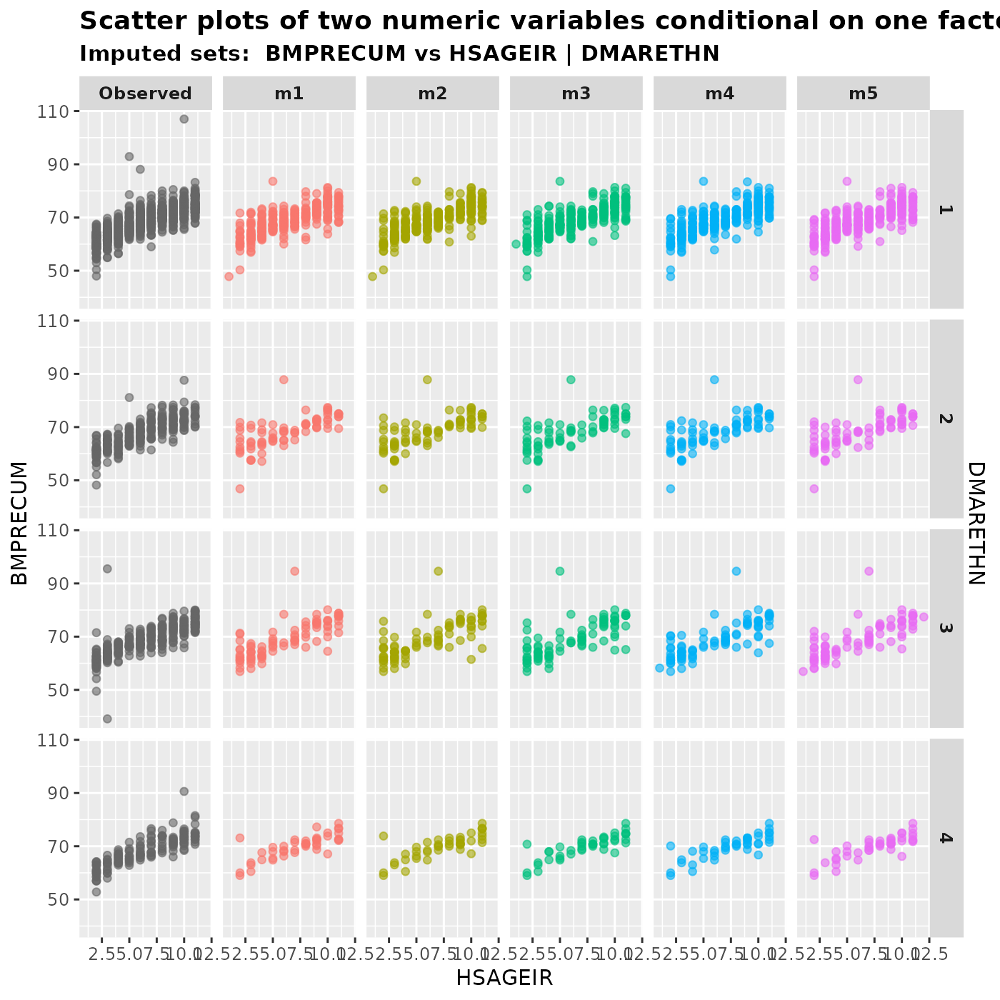
If we want to treat an integer variable as numeric, we can place it
in either var.x or var.y. Here is an example,
where HSAGEIR is an integer variable whose values range
from 2 to 11.
plot_2num1fac(
  imputation.list = imputed.data, var.x = "HSAGEIR", var.y = "BMPRECUM",
  con.fac = "DMARETHN", original.data = withNA.df
)
2.3.2 One numeric variable and one factor conditional on another factor
The function plot_1num2fac() generates boxplots with
overlaying data points for a numeric variable with a factor, conditional
on another factor.
plot_1num2fac(
  imputation.list = imputed.data, var.fac = "DMARETHN", var.num = "BMPRECUM",
  con.fac = "HSSEX", original.data = withNA.df
)
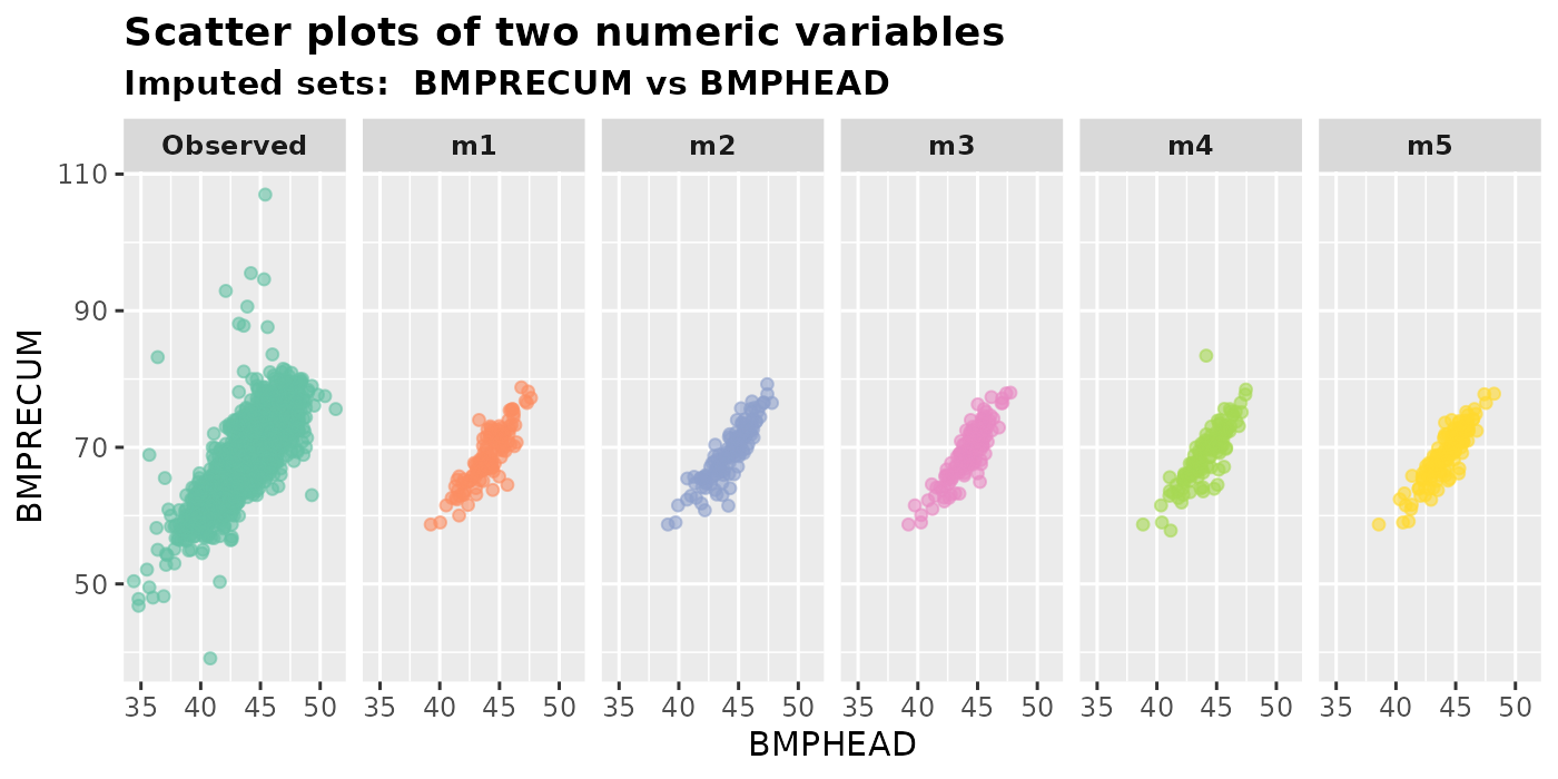
3 Color options
By default, the observed panel is gray and the other m
panels use ggplot2’s default color scheme.
plot_2num(
  imputation.list = imputed.data, var.x = "BMPHEAD", var.y = "BMPRECUM",
  original.data = withNA.df, color.pal = NULL
)
The color.pal argument allows users to specify a custom
color palette with a vector of hex codes, such as the
colorblind-friendly palette Set2 from the R package
RColorBrewer. Note that if there are m imputed
datasets, a vector of m+1 hex codes is required because an
extra color is needed for the Observed panel.
library(RColorBrewer)
color.codes <- brewer.pal(n = 6, name = "Set2")
color.codes
#> [1] "#66C2A5" "#FC8D62" "#8DA0CB" "#E78AC3" "#A6D854" "#FFD92F"

plot_2num(
  imputation.list = imputed.data, var.x = "BMPHEAD", var.y = "BMPRECUM",
  original.data = withNA.df, color.pal = color.codes
)
Otherwise, we can provide a vector of R’s built-in color names.
color.names <- c("gray50", "coral2", "goldenrod3", "darkolivegreen4", "slateblue1", "plum3")

plot_2num(
  imputation.list = imputed.data, var.x = "BMPHEAD", var.y = "BMPRECUM",
  original.data = withNA.df, color.pal = color.names
)
Here is a very useful cheat sheet of R colors names created by Dr Ying Wei.
4 Plot multiply imputed data from other packages
We can also plot multiply imputed datasets obtaining from other
packages, such as mice. Here is an example using the
nhanes2 data from mice.
This dataset consists of just 25 rows and 4 columns
(age, bmi, hyp and
chl). There are only 9, 8 and 10 missing values in the
variables bmi, hyp, and chl,
respectively. Note that imputed values are volatile when the dataset is
this small.
library(mice)
dim(nhanes2)
#> [1] 25  4
colSums(is.na(nhanes2))
#> age bmi hyp chl
#>   0   9   8  10

imp <- mice(data = nhanes2, m = 5, printFlag = FALSE)
mice.data <- complete(imp, action = "all")
plot_hist(imputation.list = mice.data, var.name = "bmi", original.data = nhanes2)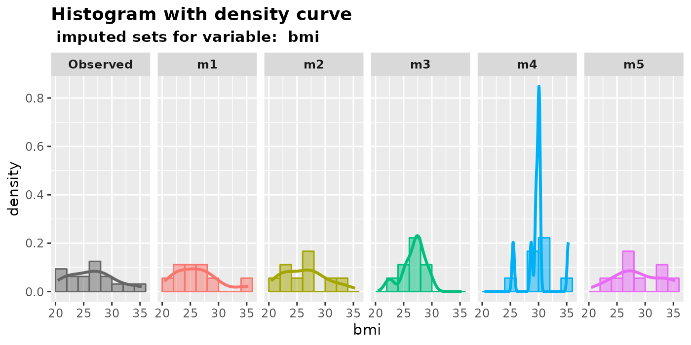
plot_box(imputation.list = mice.data, var.name = "chl", original.data = nhanes2)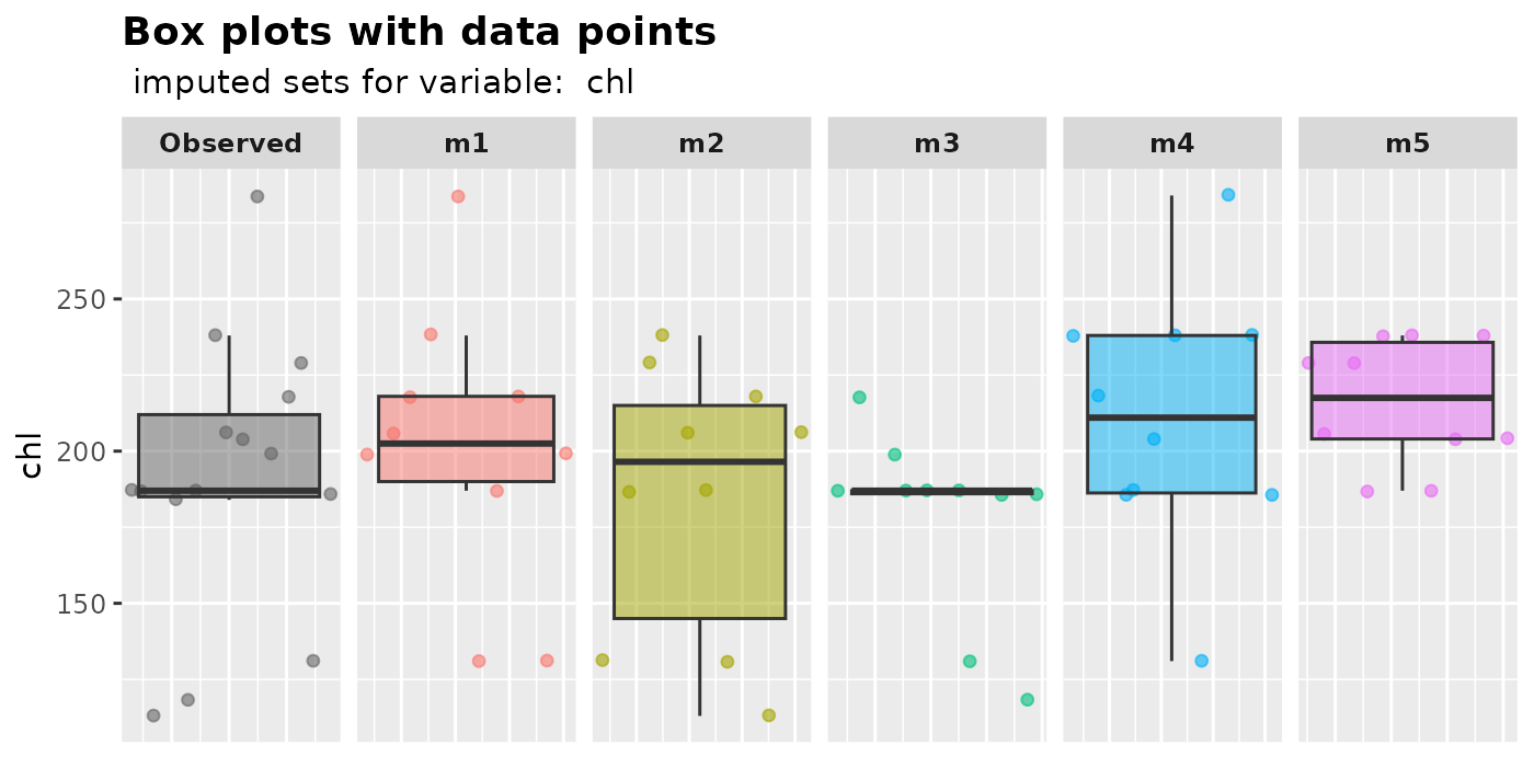
plot_bar(imputation.list = mice.data, var.name = "hyp", original.data = nhanes2)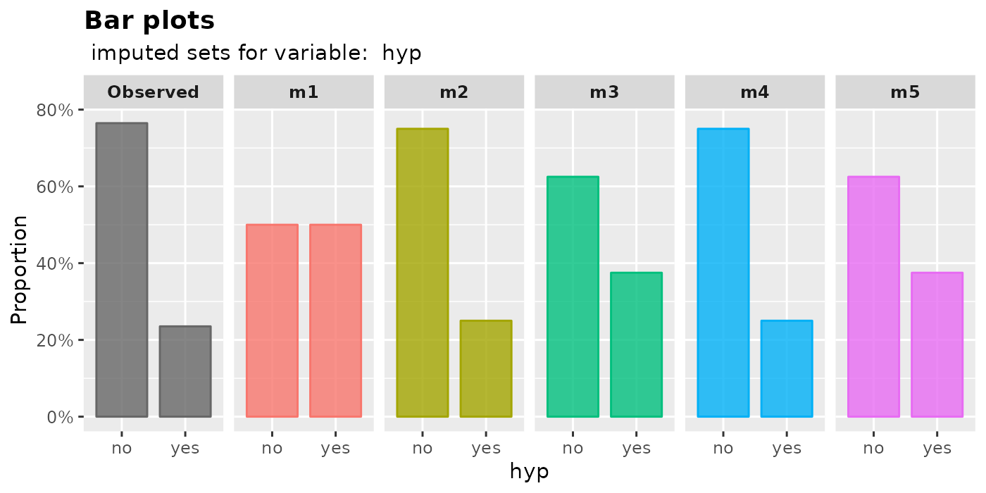
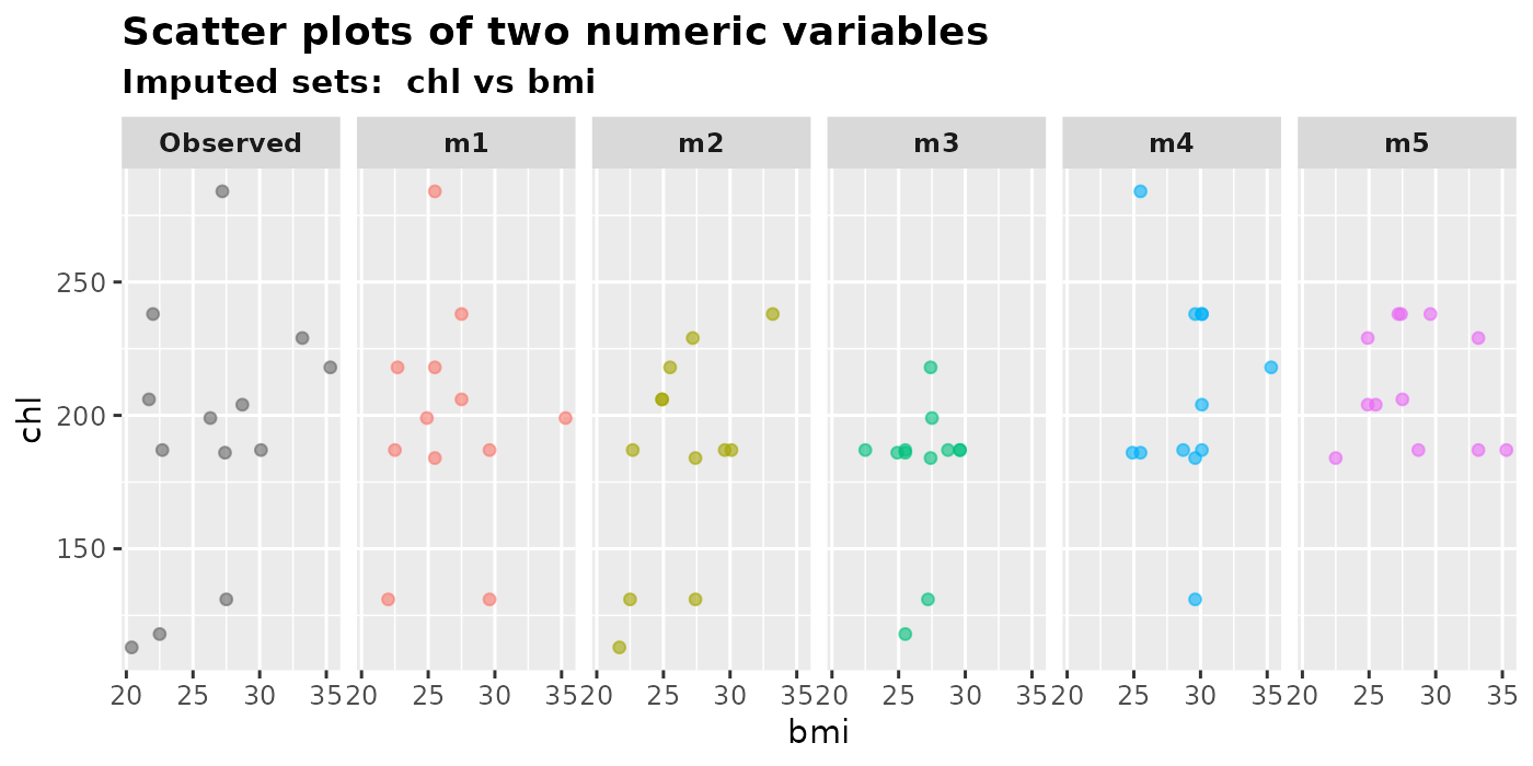
plot_2num(
  imputation.list = mice.data, var.x = "bmi", var.y = "chl",
  original.data = nhanes2
)
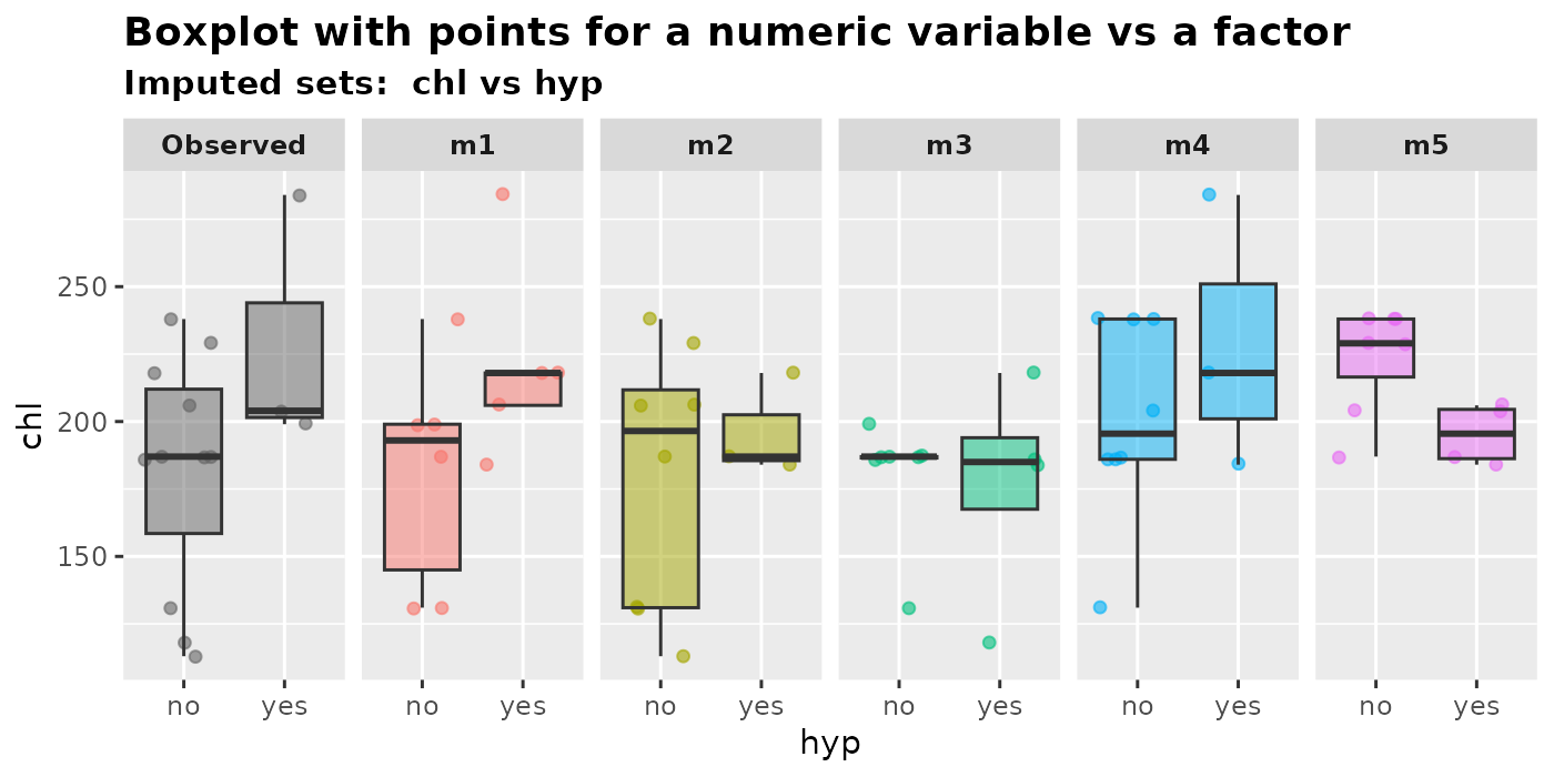
plot_1num1fac(
  imputation.list = mice.data, var.num = "chl", var.fac = "hyp",
  original.data = nhanes2
)
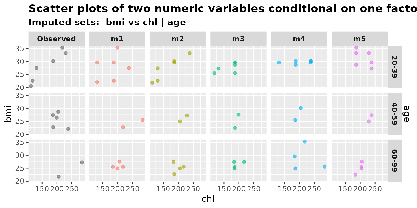
plot_2num1fac(
  imputation.list = mice.data, var.x = "chl", var.y = "bmi",
  con.fac = "age", original.data = nhanes2
)
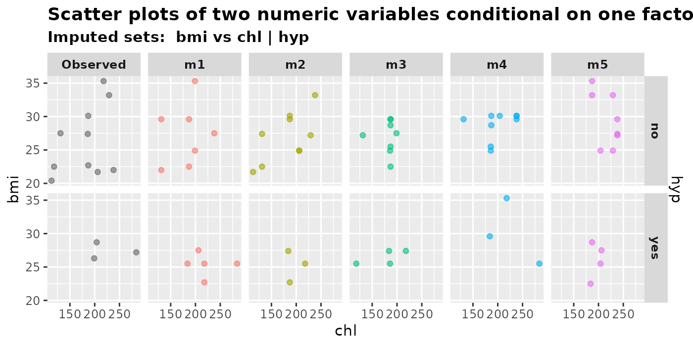
plot_2num1fac(
  imputation.list = mice.data, var.x = "chl", var.y = "bmi",
  con.fac = "hyp", original.data = nhanes2
)
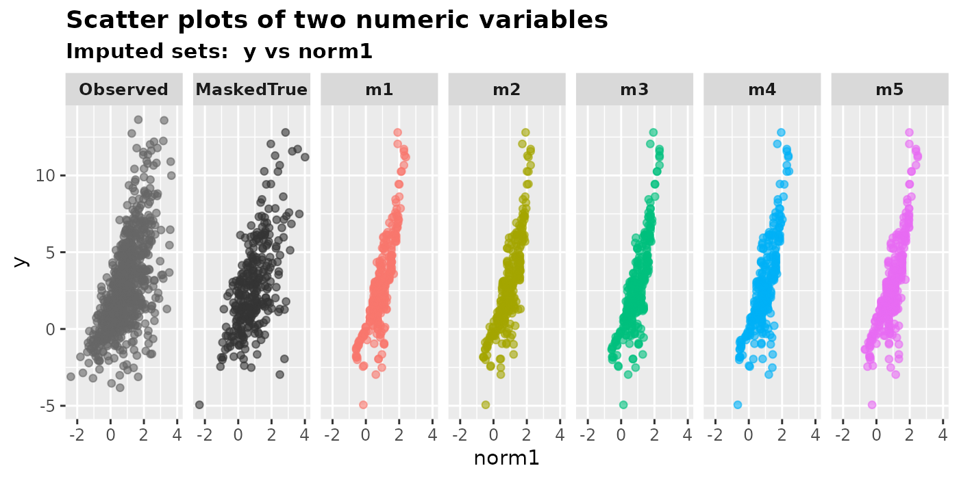
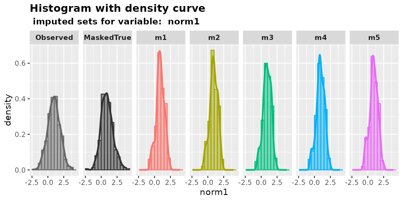
5 Plot against masked true values
In general, we do not know the true values of the missing data, thus we can only plot the imputed values versus the observed data. However, if we happen to know the true values (e.g., in cases where it is generated by simulation), we may compare them to the imputed values.
Let us generate a simple dataset full.df and create 30%
missing values in variable norm1 and norm2
under the MCAR mechanism. We then impute the MCAR.df
dataset with mixgb().
N <- 1000
norm1 <- rnorm(n = N, mean = 1, sd = 1)
norm2 <- rnorm(n = N, mean = 1, sd = 1)
y <- norm1 + norm2 + norm1 * norm2 + rnorm(n = N, mean = 0, sd = 1)
full.df <- data.frame(y = y, norm1 = norm1, norm2 = norm2)
MCAR.df <- createNA(data = full.df, var.names = c("norm1", "norm2"), p = c(0.3, 0.3))

mixgb.data <- mixgb(data = MCAR.df, m = 5, nrounds = 10)
If the true data is known, it can be specified in the argument
true.data in the visual diagnostic functions. The output
will then have an extra panel called MaskedTrue, which
shows values originally observed but intentionally made missing.
plot_hist(
  imputation.list = mixgb.data, var.name = "norm1",
  original.data = MCAR.df, true.data = full.df
)
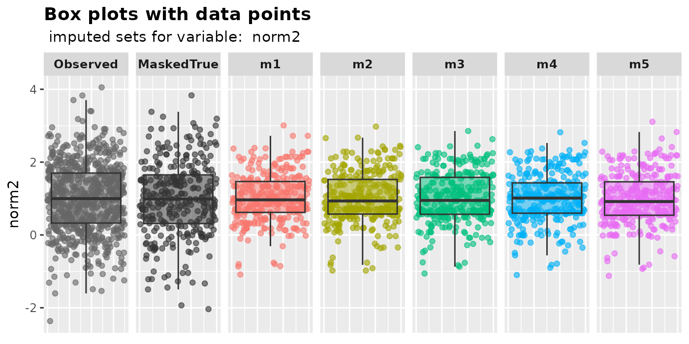
plot_box(
  imputation.list = mixgb.data, var.name = "norm2",
  original.data = MCAR.df, true.data = full.df
)
plot_2num(
  imputation.list = mixgb.data, var.x = "norm1", var.y = "y",
  original.data = MCAR.df, true.data = full.df
)